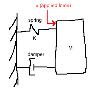
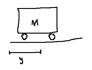
\(q \in \mathbb{R}\) is the position of the mass M
\(\dot{q} := \frac{dq}{dt}, \quad \ddot{q} := \frac{d^2q}{dt^2}\)
Assume that \(q=0\) corresponds to the mass location at which the spring is neither stretched nor compressed.
Newton's 2nd law: \(M\ddot{q} = \sum{ \text{forces acting on } M}\)
Force due to spring: \(F_K(q) = Kq\), assumed to be linear
Force due to damper, possibly nonlinear: \(C(\dot{q})\)
Altogether, we get a second order nonlinear ODE:
\[M\ddot{q} = -Kq - C(\dot{q}) + u\]
Note: if the damper is linear (\(C(\dot{q})=bq\)), then the overall system is linear
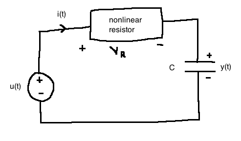
\(V_R(t) = h(i(t)), \quad h : \mathbb{R} \rightarrow \mathbb{R}\) is possibly nonlinear
\(u(t)\): applied voltage; \(y(t)\): voltage across capacitor
Apply Kirchoff's Voltage Law:
\[\begin{align}
-u(t) + V_R + y &= 0\\
\\
i(t) &= C\frac{dy}{dt} \quad \text{(capacitor equation)}\\
V_R &= h(i(t)) = h(C\dot(y))\\
\\
-u(t) + h(C\dot{y}) + y &= 0\\
\end{align}\]
Note: if the resister were linear (\(h(i) = Ri\)), the whole system would be linear (see 2.3.4 in notes)
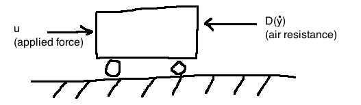
Newton's second law: \(M\ddot{y} = u - D(\dot{y})\)
We put this model into a standard form by defining two state variables:
\[x_1 := y \text{ (position)}, \quad x_2 := \dot{y} \text{ (velocity)}\]
Together, \(x_1\) and \(x_2\) make up the state of the system. We do some rewriting to have a systematic way to do linearization:
\[\begin{align} \dot{x_1} &= x_2 & \text{(state equation)}\\ \dot{x_2} &= \frac{1}{M}u - \frac{1}{M}D(x_2) & \text{(state equation)}\\ y &= x_1 & \text{(output equation)}\\ \end{align}\]
Together, these equations make up the state-space model. These equations have the general form:
\[\dot{x} = f(x,u) \text{ where } y = h(x)\]
In this example:
\[\begin{align} X &= (x_1, x_2) \in \mathbb{R}^2\\ f(x,u) &= \begin{bmatrix} x_2 \\ \frac{1}{M}u - \frac{1}{M}D(x_2) \end{bmatrix}\\ \end{align}\]
In the special case where air resistance is a linear function of \(x_2\) (\(D(x_2)=d x_2\)), then \(f(x,u)\) becomes a linear function of \(x\) and \(u\):
\[f(x,u) = \begin{bmatrix} 0 & 1 \\ 0 & \frac{-d}{M} \end{bmatrix} \begin{bmatrix} x_1 \\ x_2 \end{bmatrix} + \begin{bmatrix} 0 \\ \frac{1}{M} \end{bmatrix} u \]
Define \(C = \begin{bmatrix}1 & 0\end{bmatrix}\). In the linear case, we get:
\[\begin{align}
\dot{x} &= Ax + Bu\\
y &= Cx\\
\end{align}\]
This is a linear, time-invariant (LTI) model.
Expect at least one question like this on the midterm
Generalizing, an important class of systems have models of the form:
\[\begin{align} \dot{x} &= f(x, u), & f: \mathbb{R}^n \times \mathbb{R}^m \rightarrow \mathbb{R}^n\\ y &= h(x, u), & h: \mathbb{R}^n \times \mathbb{R}^m \rightarrow \mathbb{R}^p\\ \end{align}\]
The linear special case is:
\[\begin{align}
\dot{x} &= Ax + Bu, & A \in \mathbb{R}^{n \times m}\\
y &= Cx + Du, & C \in \mathbb{R}^{p \times m}\\
\end{align}\]
In this course, we look at single-input, single-output systems: \(m=p=1\).

\[\begin{align} m&=2, & u &= (u_1, u_2)\\ p&=2, & y &= (y_1, y_2)\\ m&=4, & x &= (x_1, x_2, x_3, x_4) := (y_1, \dot{y_1}, y_2, \dot{y_2})\\ \end{align}\]
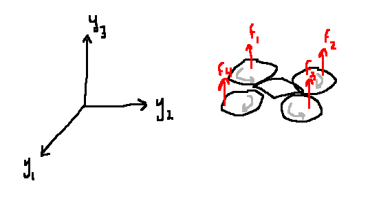
\[\begin{align}
u &= (y_1, u_2, u_3, u_4)= (f_1, f_2, f_3, f_4)\\
p&=3\\
y&=(y_1, y_2, y_3)\\
x &\in \mathbb{R}^{12} = (\text{position}, \text{orientation}, \text{velocity}, \text{angular velocity})\\
\end{align}\]
What is the state of a system?
The state vector \(x(t_0)\) encapsulates all of the system's dynamics up to time \(t_0\).
More formally: For any two times \(t_0 \lt t\), knowing \(x(t_0)\) and knowing \(\{u(t) : t_0 \le t \lt t_1\}\), we can compute \(x(t_1)\) and \(y(t_1)\).
We know \(M\ddot{y} = 0\) from Newton's laws.
If we try a 1-dimensional state, say \(x := y\), then knowing \(x(t_0)\) without knowing \(\dot{y}\) is not enough information to find the position in the future, \(x(t)\) for \(t \gt t_0\). We have the same problem if we define \(x = \dot{y}\).
Since the governing equation is second order, we need two initial conditions. So, \(x=(y, \dot{y}) \in \mathbb{r}^2\) is a good choice.
In general, it is a good idea to use:
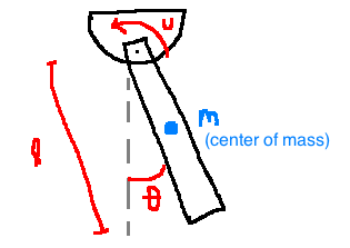
Model: \(\ddot{\theta} = \frac{3}{Ml^2} u - 3\frac{g}{l} \sin(\theta)\)
In state space form:
\[\begin{align}
x &= (\theta, \dot{\theta})\\
y &= \text{angular position} = \theta\\
\\
\dot{x}&=f(x,u) \quad & & \dot{x_1}=x_2\\
\dot{y}&=h(x,u) \quad & & \dot{x_2}=\frac{3}{Ml^2}u - 3\frac{s}{l} \sin(x_1)\\
& & & y = x_1
\end{align}\]
This is nonlinear due to the sine term.
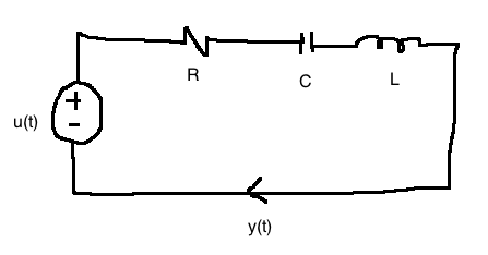
\[\begin{align} x_1 &:= \text{voltage across capacitor} = \frac{1}{C} \int{y(\tau)d\tau}\\ x_2 &:= \text{current through inductor} = y\\ \\ -u + V_R + V_C + V_L &= 0\\ \Rightarrow -u + Rx_2 + x_1 + L\dot{x_2} &= 0, \quad \text{from capacitor equation: } \dot{x_1}=\frac{1}{C} x_2\\ \\ \dot{x} &= \begin{bmatrix} 0 & \frac{1}{C}\\ \frac{-1}{2} & \frac{-R}{L}\end{bmatrix} \begin{bmatrix}x_1\\ x_2\end{bmatrix} + \begin{bmatrix}0 \\ \frac{1}{L}\end{bmatrix} u\\ y &= \begin{bmatrix}0 & 1\end{bmatrix}\\ \end{align}\]
This is the process of aproximating a nonlinear state-space model with a linear model.
Linearize \(y=x^3\) at the point \(\bar{x}=1\).
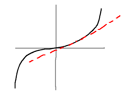
Let \(\bar{y} := f(\bar{x}) = 1^3 = 1\)
Taylor series at \(x=\bar{x}\) is:
\[y=\sum_{n=0}^\infty c_n (x-\bar{x})^n, \quad c_n = \frac{1}{n!} \frac{d^n f(x)}{dx^n} \biggr|_{x=\bar{x}}\]
Keep only the terms \(n=0\) and \(n=1\):
\[\begin{align}
f(x) &\approx f(\bar{x}) + \frac{df(x)}{dx}\biggr|_{x-\bar{x}} (x-\bar{x})\\
y - \bar{y} &\approx + \frac{df(x)}{dx}\biggr|_{x-\bar{x}} (x-\bar{x})\\
\end{align}\]
If we define the derivations \(\partial y := y - \bar{y}, \partial x := x - \bar{x}\), then \(\partial y = \frac{df}{dx} \bigg|_{x=\bar{x}} \partial x\), i.e. \(\partial y = 3 \partial x\)
\[y = \begin{bmatrix}y_1 \\ y_2\end{bmatrix} = f(x) = \begin{bmatrix}x_1 x_2 - 1 \\ x_3^2 - 2x_1 x_3\end{bmatrix} =: \begin{bmatrix}f_1(x) \\ f_2(x)\end{bmatrix}\]
Linearize at \(\bar{x}=(1, -1, 2)\).
\(\bar{y}=f(\bar{x})=\begin{bmatrix}-2\\0\end{bmatrix}\)
\[d(x)=f(\bar{x})+\frac{\partial f}{\partial x} \biggr|_{x=\bar{x}} (x-\bar{x}) \text{ + higher order terms}\]
The Jacobian of \(f\) at \(\bar{x}\) is:
\[\begin{align}
\frac{\partial f}{\partial x} \biggr|_{x = \bar{x}}
&= \begin{bmatrix}
\frac{\partial f_1}{\partial x_1} & \frac{\partial f_1}{\partial x_2} & \frac{\partial f_1}{\partial x_3} \\
\frac{\partial f_2}{\partial x_1} & \frac{\partial f_2}{\partial x_2} & \frac{\partial f_2}{\partial x_3} \\
\frac{\partial f_3}{\partial x_1} & \frac{\partial f_3}{\partial x_2} & \frac{\partial f_3}{\partial x_3} \\
\end{bmatrix}\\
&= \begin{bmatrix}
x_2 & x_1 & 0 \\
-2x_3 & 0 & 2x_3-2x_1 \\
\end{bmatrix}_{x=(1, -1, 2)}\\
&= \begin{bmatrix}
-1 & 1 & 0\\
-4 & 0 & 2
\end{bmatrix}\\
&= A
\end{align}\]
i.e. \(y-\bar{y} \approx A(x-\bar{x})\)
By extension, near \((x,u)=(\bar{x}, \bar{u})\):
\[f(x, u) \approx f(\bar{x}, \bar{u})+ \frac{\partial f}{\partial x} \biggr|_{(x,u)=(\bar{x}, \bar{u})} (x-\bar{x}) + \frac{\partial f}{\partial u} \biggr|_{(x,u)=(\bar{x}, \bar{u})} (u-\bar{u})\]
Let's apply this to \(\dot{x}=f(x,u), y=h(x,u)\).
Definition: A constant pair \((\bar{x}, \bar{u}) \in \mathbb{R}^n \times \mathbb{R}^m\) is an equilibrium configuration of the system \(\dot{x}=f(x,u), y=h(x,u)\) if \(f(\bar{x}, \bar{u})=(0,...,0)\). The constant \(\bar{x}\) is the equilibrium point.
\[\begin{align} \dot{x} &= f(x,u)\\ y &= h(x,u)\\ x_1 &= \theta\\ x_2 &= \dot{\theta}\\ f(x,u) &= \begin{bmatrix}x_2\\ \frac{3}{Ml}u-\frac{3g}{l}\sin(x_1)\end{bmatrix}\\ h(x) &= x_1 \end{align}\]
If \(y=\pi\) (upright), then \(\bar{x_1}=\pi\). So we have to solve:
\[
\begin{bmatrix}0\\0\end{bmatrix} = \begin{bmatrix}
\bar{x_2}\\
\frac{3\bar{u}}{Ml} - \frac{3g}{l}\sin(\bar{x_1})
\end{bmatrix} \Rightarrow \bar{x_2}=0, \quad \bar{u}=0
\]
Therefore the equilibria are:
\[
\begin{bmatrix}\bar{x_1}\\\bar{x_2}\end{bmatrix} = \begin{bmatrix}\pi + 2\pi k \\ 0\end{bmatrix}, \quad \bar{u}=0
\]
Assume that \(\dot{x}=f(x,u)\) has an equilibrium configuration at \((x,u)=(\bar{x}, \bar{u})\).
\[ f(x,u) \approx \underbrace{f(\bar{x}, \bar{u})}_{=0} + \underbrace{\frac{\partial f}{\partial x} \biggr|_{(x,u)=(\bar{x}, \bar{u})} (x - \bar{x})}_{=: A} + \underbrace{\frac{\partial f}{\partial u} \biggr|_{(x,u)=(\bar{x}, \bar{u})} (u - \bar{u})}_{=:B}\]
Consider deviations from \((\bar{x}, \bar{u})\), where \(||\partial x||, ||\partial u||\) are assumed to be small:
\[\begin{align}
\partial x(t) &:= x(t) - \bar{x}\\
\partial u(t) &:= u(t) - \bar{u}\\
\end{align}\]
Then we get linearized state equations:
\[\dot{\partial x} = \dot{x} - 0 = f(x,u) \approx A\partial x + B \partial u\\
\dot{\partial x} = A\partial x + B\partial u\]
Linearized output equation:
\[\partial y = \underbrace{\frac{\partial h}{\partial x} \biggr|_{(x,u)=(\bar{x},\bar{u})} \partial x}_{=:C} + \underbrace{\frac{\partial h}{\partial u} \biggr|_{(x,u)=(\bar{x},\bar{u})} \partial u}_{=:D}\\ \partial y := y-\bar{y}=y-h(\bar{x},\bar{u})\]
Linearizing \(\dot{x}=f(x,u)\) and \(y=h(x,u)\):